3D Autotiling: Basic WFC

Introduction

#

I don’t think I would have become interested in shooters if it weren’t for Halo 3’s forge mode. I probably logged 1000 hours in Minecraft when I was a kid (and learned Java because of it!). Games that let you make stuff are the best. Making games is even better. After a few years focusing on my career in network programming I decided to revisit games, this time looking at 3D.

I picked up a book on 3D modeling and then tried to start making a game. Building a castle felt a bit tedious to me, even with a modular kitbash asset pack. In 2D and 3D, I hate rotating and aligning tiles to fit.

In Townscaper, it’s very easy to build something that looks “correct”. I wanted to replicate that experience in a level editor. This led me down a rabbit hole into exploring different procedural generation techniques: Wave Function Collapse, Marching Cubes for terrain, Heightmap Terrain. The hardest part was modifying them to make them artist controllable.

This short series covers my Wave Function Collapse implementation. I’ve implemented the core algorithm 4 times. First in Blender/Python intending to export to Unity/C#. Unity had issues on my Linux machine so I tried Bevy/Rust. Turns out an editor is a valuable debugging tool and I finally have a solid working version in Godot.

2D Autotiling with Marching Squares

#

There are lots of better choices for 2D autotiling. This tutorial is a baby step towards what I truly want to show.

Marching Squares and it’s 3D cousin Marching Cubes are both algorithms for converting an array of scalar values into a shape or mesh. These algorithms are pretty robust and with high enough resolution and smart interpolation, they will produce a very nice output.

Both algorithms operate on a dual grid. You can think of this as having a secondary grid offset by half a cell. I prefer to imagine the cells as containing data and the corners of the cells containing separate but related data. In this case, the corners of the grid represent the “density” information. That could be a ‘0meaning "empty," or a1` indicating “filled.” If we want a smoothed result, we could use an arbitrary scalar value telling us how full it is.

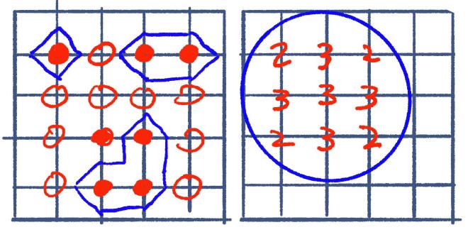
The goal here is 2D auto-tiling, not generating a smooth mesh. So we can treat the corners as either filled or empty. We have four corners per cell with two possibilities. That’s 2⁴ (16) total combinations.

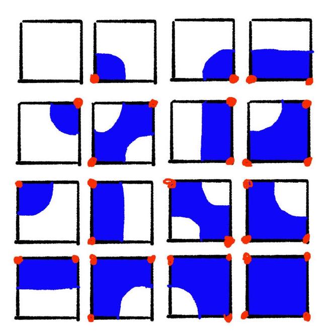
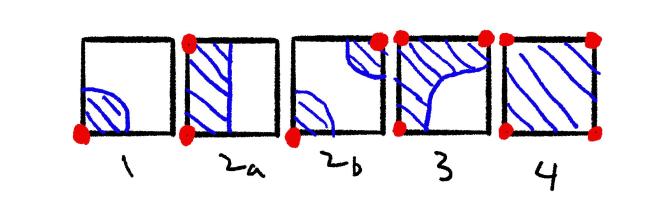
Depending on the art style, you may not need unique tiles for the same shape in different directions. If we remove cases that are mirrors or rotations of others, we only have five things to draw. Notice that in that 2b, the diagonal case can either be a gap or a bridge. In marching squares, this is called a saddle point. We’re just going to make that an artistic/gameplay choice here.

For this tutorial, I’m going to use Godot with GDScript. Feel free to follow along with whatever you’re comfortable with.

Lookup Table

#

We can think of each corner as one bit of a 4-bit integer. Starting in the top left, moving in clockwise order, we will set the least significant bit for each “filled” corner.

var lookup = {
	# empty
	0: {"tile": 0, "rotation": 0}, 

	# corner 
	1: {"tile": 1, "rotation": 0},
	8: {"tile": 1, "rotation": 1},
	4: {"tile": 1, "rotation": 2},
	2: {"tile": 1, "rotation": 3},

	# edge 
	3: {"tile": 2, "rotation": 0},
	6: {"tile": 2, "rotation": 3},
	9: {"tile": 2, "rotation": 1},
	12: {"tile": 2, "rotation": 2},

	# diagonal 
	5: {"tile": 3, "rotation": 0},
	10: {"tile": 3, "rotation": 1},

	# bend
	7: {"tile": 4, "rotation": 0},
	11: {"tile": 4, "rotation": 1},
	13: {"tile": 4, "rotation": 2},
	14: {"tile": 4, "rotation": 3},

	# full
	15: {"tile": 5, "rotation": 0},
}

Cursor

#

Pretty simple:

func _ready():
	cursor = ColorRect.new()
	cursor.color = Color(1, 0, 0, 0.5)
	cursor.size = Vector2(TILE_SIZE, TILE_SIZE)
	add_child(self.cursor)

func _input(event):
	if event is InputEventMouse:
		var rounded = Vector2i(event.position / TILE_SIZE) * TILE_SIZE
		self.cursor.position = rounded
		if event is InputEventMouseButton and event.is_pressed():
			_toggle(rounded)

Bit Flipping

#

First we add a top level dictionary:

// Vector2i -> int
var tiles = {}

We will key the dictionary by the Vector2i coordinate where we want to draw the tile. The value is the index to use in the lookup table. We will mani

We manipulate the index at the four surrounding coordinates when we click on the grid. We can think of the coordinates we click on as the “corners” or the “dual grid” of the grid that tiles draw. The bit we change must correspond to the corner of the tile grid cell on which this “dual” coordinate lies. Since the bottom right corner uses the the first bit, we start with that and then go counterclockwise.

var offsets =  [
	Vector2i(1, -1),
	Vector2i(0, -1),
	Vector2i(0, 0), 
	Vector2i(1, 0), 
]

func _toggle(pos: Vector2i):
	var grid_coord = pos / TILE_SIZE
	
	for i in range(len(offsets)):
		var offset_coord = grid_coord + offsets[i]
		if offset_coord not in tiles:
			tiles[offset_coord] = 0
		tiles[offset_coord] ^= 1 << i

Lookup and Draw

#

Finally, we can do a lookup using the index which we just modified.

func _toggle(pos: Vector2i):
    ...
    for i in range(len(offsets)):
        # flip a bit 

    	var s = get_node_or_null(str(offset_coord))
		if not s:
			s = Sprite2D.new()
			s.name = str(offset_coord)
			s.texture = tileset
			s.region_enabled = true
			s.position = (offset_coord + Vector2i.DOWN) * TILE_SIZE
			add_child(s)
		
		if tiles[offset_coord] == 0:
			s.queue_free()
		else:
			var tile = lookup[tiles[offset_coord]]		
			s.region_rect = Rect2(tile["tile"] * TILE_SIZE, 0, TILE_SIZE, TILE_SIZE)		
			s.rotation_degrees = 90 * tile["rotation"]

Pretty simple. Less than 100 lines of code and we have a working demo. Extending this to 3 dimensions isn’t difficult. Instad of each cell having four corners, it has 8. The hard part is building a tileset and lookup table that can support 2⁸ (256) possibilities.

Basic Wave Function Collapse

#

This 3D autotiling project started when I stumbled on Martin Donald’s Wave Function Collapse video. He explained it so well that I had to try it out.

In this post I will attempt to outline the high-level structure of a Wave Function Collapse implementation with a bit of pseudo-Python. This is not a tutorial, but more of a brief recap of my first implementation from over a year ago.

Algorithm

#

The algorithm has two main phases: Collapse and propagation. Collapse is a cute name for picking a value for some cell. When we observe the cell reduces its superposition of possible states into a single value. Propagation is where we use that definite value to narrow down the possible values of neighboring cells.

We start with a grid and a tileset. Each cell of the grid contains all of the tiles as its possibilities.

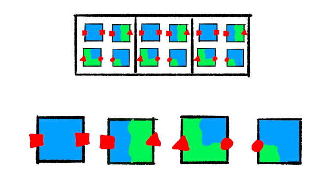
Next, we pick a random tile for one of the cells. Because the “square” socket is on the right side of the tile we picked, the next cell can only contain tiles that match that socket on the adjacent side. That propagates out into the third cell as well. Our middle cell only exposes a triangle and a square so the tile with a circle on the left gets eliminated.

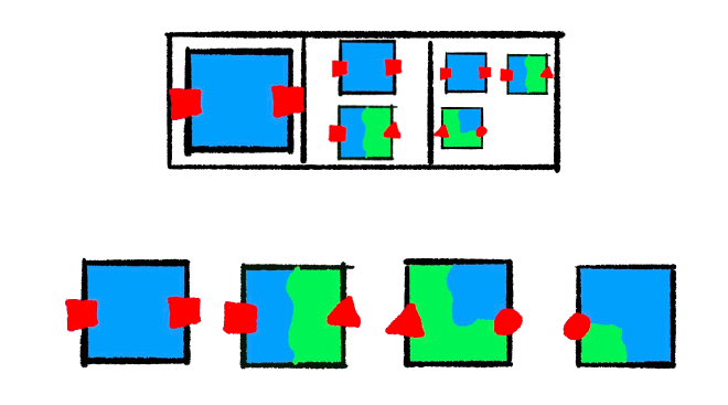
From this state, if we choose the “edge” tile with the triangle socket for the middle cell there is only one compatible tile in the rightmost cell, therefore the grid is solved. If we choose another completely blue tile here, we must make one more choice.

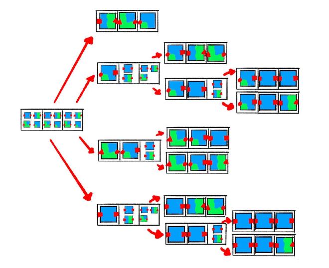
We end up with a solid number of possible final states even in our limited example. The number of choices is less than or equal to the number of cells. In practice, we rarely make a random choice for the majority cells. After a few essential cells are collapsed, the propagation step chooses by process of elimination. The worst case, performance-wise, is if we have so many compatible tiles that we don’t quickly prune possibilities in the first few iterations.

Types

#

I have a handful of foundational structures in my implementation.

Prototypes

#

class Prototype:
    name: str
    mesh: str
    rotation: int

    # sockets
    north: str
    east: str
    south: str
    west: str
    top: str
    bottom: str

A prototype represents a possible choice to put somewhere in the grid. We will have 4 prototypes for each tile in our tileset, one for each 90-degree rotation.

Sockets

#

On each of the 6 faces we will have a socket. These identify which Prototypes can connect to each other in each direction. The socket represents what we see when we look at one face of the tile’s bounding box.

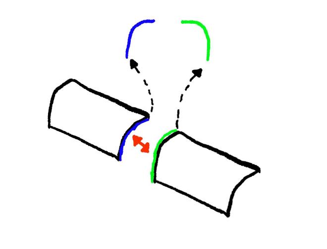
For the north and south or east and west sockets to match, they must be mirrors of one another. For a vertical face’s socket to fit the sockets must be identical. Sockets are arbitrary strings, except for the suffixes on horizontal faces’ sockets: s (symmetrical) and f (flipped).

def compatible_sockets(face, a, b) -> bool:
    # symmetrical faces should be identical
    if face in {"top", "bottom"} or a.endswith("s"):
        return a == b     
    flipped_b = socket[:-1] if socket.endswith("f") else b + "f"
    return a == flipped(b)

Cells

#

class Cell:
    possibilities: list[Prototype]

A cell is one element in a Grid, which is just a collection of Cells.

Grid

#

How you represetnt a Grid depends on your application. BorisTheBrave wrote an entire C# library, Sylves, for handling grids.

It could be a 3D array:

class Grid:
    grid: list[list[list[Cell]]]

Or for an infinite grid, a map that lazily populated:

class Grid:
    grid: dict[Vec3, Cell]

    def __getitem__(self, coord: Vec3):
        if key not in self.grid:
            self.grid[coord] = Cell()
        return self.grid[coord]

Our only requirement is that we can use a 3D coordinate as a key.

Implementation

#

def solve():
    work_list = []
    solved = False
    iteration = 0
    while not solved and iteration < MAX_ITERATIONS:
        iteration += 1

        cell, coord = grid.find_min_entropy()
        if cell is None:
            solved = True
            break

        cell.collapse()
        work_list.append(coord)
        while len(work_list) > 0:
            work_list += propagate(work_list.pop())

Here is the algorithm we described earlier:

1. Make a random selection in one of the cells
2. Recursively propagate that out and repeat until every cell has only one possibility.

You can perform the selection bit by hand in this web demo from Martin Donald.

Collapse

#

In this algorithm, “entropy” is a cute name for the length of a Cell’s possibility list. Zero means there is a contradiction and we will never be able to solve the Grid. One means we have already chosen the Prototype for this cell. In each iteration, we find the unsolved Cell we’re most certain about:

def min_entropy(self) -> Cell:
    def entropy(cell):
        if cell.entropy() < 2:
            return math.inf
        return cell.entropy()
    return min(self.grid, key=entropy)

Then we “collapse” its possibilities into a random choice:

def collapse(self):
    idx = randint(0, len(self.possibilities) - 1)
    self.possibilities = [self.possibilities[idx]]

Propagate

#

def propagate(coord):
    cur_cell = self.grid.get(cur_coord)
    changed_neighbors = []
    for direction in opposing_faces.keys():
        next_coord = add_vec3(cur_coord, face_deltas[direction])
        if not self.grid.is_in_bounds(next_coord):
            continue
        next_cell = self.grid.get(next_coord)
        changed = grid[next_cell].constrain_to_neighbor(cur_cell, direction)
        if changed:
            changed_neighbors.append(next_coord)
            self.propagation_stack.append(next_coord)
    return changed_neighbors

Any time we change the possibility list of one cell, the neighboring cells are possibly affected. We reduce the possibility list of each adjacent cell with constrain_to_neighbor, and if that causes a change, we will have to propagate to that cell’s neighbors as well.

Constrain

#

def constrain_to_neighbor(self, cell: Cell, face: str):
    old = len(self.possibilities)
    self.possibilities = [
        p
        for p in self.possibilities[]
        if compatible_sockets(my_face, p[my_face], cell[face])
    ]
    return old != len(self.possibilities)

Here, we reduce the possibility list to only include Prototypes that are compatible on the opposing face.

There are far more efficient ways of doing this, like setting up an adjacency table. This is also the part of the algorithm that will most likely have edge cases to help guide the algorithm’s behavior to produce specific results.

Generating Sockets and Prototypes

#

Sockets from Geometry

#

To use the algorithm above will need to label each of our tiles with sockets. We could do this by hand. 16 meshes, multiplied by their 6 cell faces 96 labels would need to be written out. Why spend twenty minutes doing something tedious when you can spend a couple hours automating it?

My strategy for automating this is to filter the vertices to only those that sit on the face of the tile’s bounding box, and generate a hash to use as the socket. There are some special considerations, though:

1. We need to know if a socket is a mirror of another socket.
2. If we want rotated Prototypes, we need to be able to rotate a socket.
3. For faces with no vertices, we must know if they’re inside pieces or outside pieces, otherwise we might expose some backfaces instead of generating something manifold.

Using a hash alone won’t cut it; we would lose the vertex info. To handle this we can map the hash to some friendly name, and use suffixes to indicate these things.

1. f - a flipped version of a socket
2. s - a socket that is symmetrical (no need to flip)
3. r0, r1, r2, r3 - number of 90 rotations done to a socket

We’re also going to have to look at some normal data to cover that “empty” socket scenario.

Using the mesh data is pretty finnicky. It’s hard to tell what direction things are facing reliably. The requirements put on the artist to make near perfect meshes are also very annoying. For high poly meshes, the implementation I have here would be slow or not even work. I ended up mostly abandoning this approach. I’ll get into that in a later post.

The implementation can be found here along with a sample Blender file you can use to run the code. Rather than walking through the entire thing, I’ll highlight some semi-interesting bits.

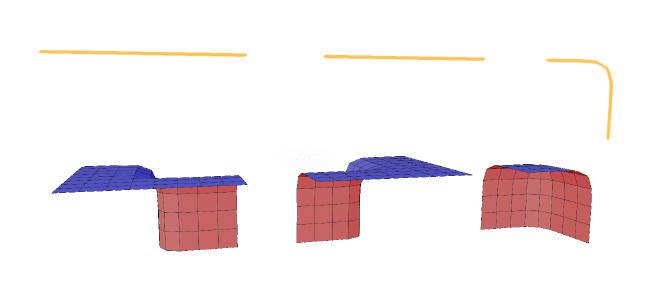
Detecting Interiors

#

def is_interior(o: bpy.types.Object, face):
    axis, sign = get_axis(face)
    detected_sign = 0
    max_poly = -float("inf")
    for p in o.data.polygons:
        normal = Decimal(f"%.{DECIMAL_PLACES}f" % p.normal[axis])
        if normal.is_zero():
            continue

        normal_sign = 1 if normal > 0 else -1
        for vert_idx in p.vertices:
            vert_value = sign * o.data.vertices[vert_idx].co[axis]
            if vert_value > max_poly:
                detected_sign = normal_sign
                max_poly = vert_value

    return detected_sign != sign:

I’m just finding the mesh face that’s furthest in the axis for our tile face (north, west, top, etc.), and seeing if its normal matches that direction.

This is a simplistic method that’s prone to errors. It’s good enough for because the meshes are so simple. The plan was that I would run this on the simple versions, and then re-use that data after I add details and art to the meshes.

Conclusion

#

While this post was mostly pseudo code, it matches up pretty well to my first WFC attempt. The code is available here as well as a sample Blender file you can use to run it. This implementation has majorissues and isn’t scalable, but I found I use for it that’s covered in a later post.